Neural Network Optimization Algorithms Explained with Code

9 minute read

Optimization algorithms play a major role in Deep Learning. After all, if our neural networks don’t learn anything, they are hardly useful. There is a whole suite of algorithms that people have come up with throughout the years to optimize the parameters of a neural network in order to minimize loss functions. Many articles I found about this topic focus solely on the mathematics behind these algorithms, making it really hard for beginners to grasp the concepts. Out of all the explanations I saw so far, my favorite one was given by Justin Johnson in this video of Stanford’s CS231n, a course on Deep Learning for Computer Vision. It combines intuitive explanations of the mathematical concepts with short code snippets, making it easy to understand how these algorithms work. In this article, my goal is to give equally intuitive explanations for the five common optimization algorithms that are also covered in the linked video: Stochastic Gradient Descent (SGD), SGD with momentum, AdaGrad, RMSProp, and Adam. So let’s begin.

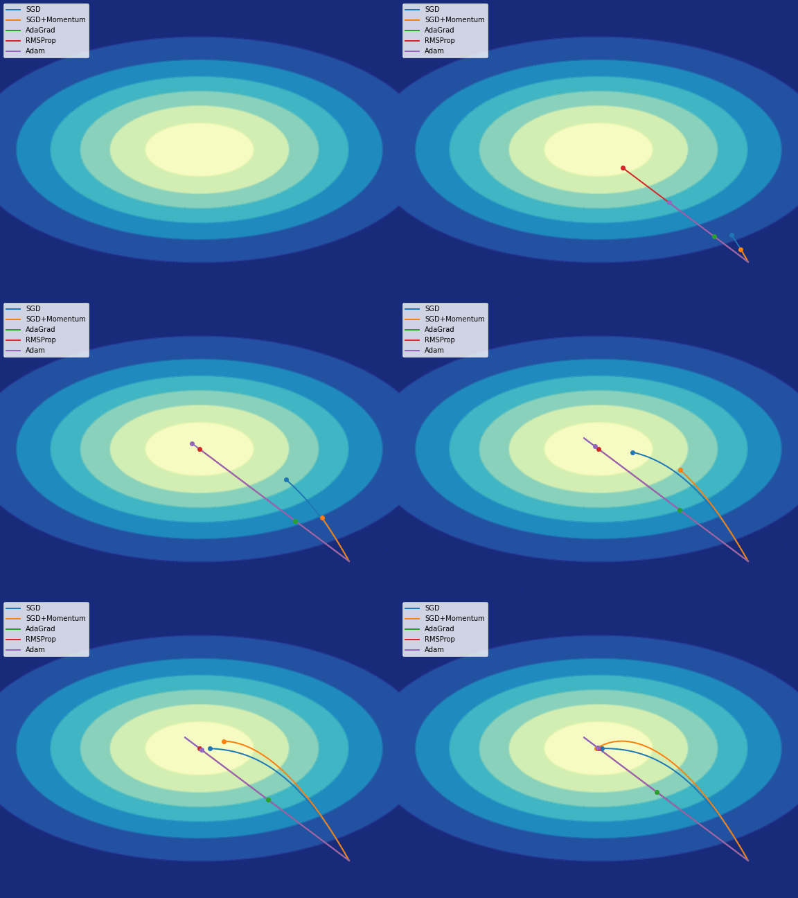
To start with, it is always worthwhile noting how important it is to implement these algorithms yourself and experiment with them. Although their concepts can be expressed with just a handful of formulas and a couple lines of code, it took me a few hours to get all the details right when trying to produce a visualization like this one:

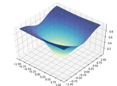
The code for reproducing the plots in this post can be found on my GitHub. I used the TrajectoryAnimation class from Louis Tiao’s blog post to construct the animation. For my experiments, I chose a simple two dimensional function with a Gaussian shape:

$f(x, y) = -e^{-(\frac{x^2}{0.7} + \frac{y^2}{0.3})} + 1$

This function’s minimum is at $f(0, 0) = 0$, which is right in the center in the plot above.

Stochastic Gradient Descent (SGD)

Gradient Descent forms the basis for all the algorithms covered in this article. SGD is thus the most vanilla algorithm to perform neural network optimization. The concept can be explained with a single simple formula:

$x_{t+1} = x_t - \alpha\nabla f(x_t)$

Where $\alpha$ is what is referred to as the learning rate and $\nabla f(x_t)$ is the gradient of $f$ at position $x_t$. The algorithm’s representation in code is just as simple:

def sgd(x, learning_rate=1e-2, num_steps=100):
    for i in range(num_steps):
        dx = compute_gradient(x)
        x -= learning_rate * dx
    return x

Here, compute_gradient is an ominous function that computes the gradient of our function of interest $f$ at the given position $x$. We can derive the gradient for our function above analytically:

$\nabla f(x, y) = \begin{pmatrix} \frac{\partial f}{\partial x} \\ \frac{\partial f}{\partial y} \\ \end{pmatrix} = \begin{pmatrix} \frac{2x}{0.7}e^{-(\frac{x^2}{0.7} + \frac{y^2}{0.3})} \\ \frac{2y}{0.3}e^{-(\frac{x^2}{0.7} + \frac{y^2}{0.3})} \\ \end{pmatrix}$

Now we can fill in the values for $x$ and $y$ at our current position and obtain the gradient. The gradient always points in the direction of steepest ascent of a function. Thus, to minimize the function $f$, we take a step in the opposite direction of the gradient. To make sure that we don’t overshoot our target location of $(0, 0)$ by taking a huge step, we multiply the gradient by the learning_rate in order to approach our target location little by little.

This seems like a good approach. However, there are several problems with vanilla SGD. In regions where the function is very flat, the gradient will be almost zero. This problem gets especially apparent in high dimensions, where saddle points can occur more often.

Another problem occurs when the target function changes quickly in one direction and slowly in another. Justin Johnson uses the metaphor of a taco shell to visualize this. With such a function, the gradient in the steep direction would be very large, while the gradient in the shallow direction would be much smaller. This causes a sort of zigzagging behavior of the optimization algorithm along the steep direction, while the progress we make towards the minimum with each step is very small.

Since we usually train our neural networks on randomly sampled mini-batches, the gradients we compute are stochastic, which also means that they are only a noisy approximation of the true gradient. This can cause SGD to take even longer to reach the minimum.

SGD+Momentum

By adding the concept of velocity or momentum to the SGD algorithm, we are able to overcome some limitations of the vanilla implementation. The mathematical formulation for SGD with momentum is just marginally more complex than before:

$v_{t+1} = \rho v_t + \nabla f(x_t) \\ x_{t+1} = x_t - \alpha v_{t+1}$

Where $\rho$ corresponds to a constant that represents some sort of friction. A simple implementation of SGD with momentum could look like this:

def sgd_momentum(x, learning_rate=1e-2, momentum=0.9, num_steps=100):
    vel = np.zeros(x.shape)
    for i in range(num_steps):
        dx = compute_gradient(x)
        vel = momentum * vel + (1 - momentum) * dx
        x -= learning_rate * vel
    return x

With momentum, we build up velocity as a running mean of the gradients. Typical values for the momentum term are 0.9 or 0.99. At every update step, the current velocity is decayed by the friction constant, and the new gradient is added in. Afterwards, we take a step into the direction of the velocity, rather than stepping in the direction of our actual gradient like before.

There are a few things to note here. You will likely come across different ways to calculate the velocity. In this implementation, I used (1 - momentum) as a dampening factor for dx before adding it to the decayed velocity. PyTorch’s implementation of SGD lets you specify a separate dampening factor in addition to the momentum parameter. In the Stanford lecture linked above, you will see that the gradient is incorporated into the velocity without any dampening. Which one you choose ultimately depends on your specific problem. As can be seen in the animation in the beginning of this post, using (1 - momentum) causes the optimizer to take quite some time to build up speed, which is why it lags behind the vanilla implementation of SGD. However, keep in mind that the optimization problems we try to solve when training Neural Networks are not as trivial as shown in this animation. The main intention of incorporating momentum in the update step is that of being able to “roll past” flat areas with low gradients, just like a ball rolling down a hill. Additionally, in scenarios like the taco shell example mentioned before, the momentum will ideally cause the gradients along the steep dimension to cancel out, so that we can continue to accumulate speed into the direction of the actual minimum.

AdaGrad

In AdaGrad, instead of having a velocity term, we keep a running sum of the squared gradients during training. Afterwards, we divide our current gradient by the square root of the squared gradient sum. We add a tiny 1e-8 term to the denominator to make sure that we don’t divide by zero. All of this can be expressed with just a minor modification to the code of the SGD optimizer:

def ada_grad(x, learning_rate=1e-2, num_steps=100):
    grad_squared = np.zeros(x.shape)
    for i in range(num_steps):
        dx = compute_gradient(x)
        grad_squared += dx * dx
        x -= learning_rate * dx / (np.sqrt(grad_squared) + 1e-8)
    return x

This division at the end has an interesting effect. Say we have a gradient that is very large in some components, and very small in others. As we accumulate the sum of squared gradients and then divide our current gradient by that sum, the large components in the gradient are divided by a large number, while the small components are divided by a small number. This effectively lets us accelerate our movement along the dimensions in which the gradient is small, while it slows down the movement along the dimensions with a large gradient, thus reducing jitter in the gradient updates just like SGD with momentum.

However, as the training progresses, we keep adding gradients to our sum. Since we divide the step size by this sum, the parameter updates will just become smaller and smaller. This can be seen in the animation above, in which the progress that AdaGrad makes slows down gradually. One can try countering this effect by fine-tuning the learning rate, but it turns out that in practice there are other methods like RMSProp and Adam that accommodate for this issue.

RMSProp

RMSProp addresses AdaGrad’s problem of accumulating the squared gradients by introducing a decay factor. The calculation of the squared gradients now looks very similar to the calculation of the momentum in SGD:

def rms_prop(x, learning_rate=1e-2, beta=0.99, num_steps=100):
    grad_squared = np.zeros(x.shape)
    for i in range(num_steps):
        dx = compute_gradient(x)
        grad_squared = beta * grad_squared + (1 - beta) dx * dx
        x -= learning_rate * dx / (np.sqrt(grad_squared) + 1e-8)
    return x

Instead of keeping a running average of the gradients, RMSProp keeps a running average over the squared gradients. At each step, we decay the previous estimate of the squared gradients by beta and add in (1 - beta) of the current squared gradient. The change from AdaGrad to RMSProp is minimal, but the effect is huge, since the parameter updates do not slow down anymore, as you can see in the animation above.

Adam

Adam combines SGD with momentum and RMSProp by maintaining a weighted sum of the gradients and a weighted sum of the squared gradients. We call these the first and second moments. In code, this looks something like this:

def adam(x, learning_rate=1e-2, beta1=0.9, beta2=0.999, num_steps=100):
    first_moment = np.zeros(x.shape)
    second_moment = np.zeros(x.shape)
    for i in range(num_steps):
        dx = compute_gradient(x)
        first_moment = beta1 * first_moment + (1 - beta1) * dx
        second_moment = beta2 * second_moment + (1 - beta2) * dx * dx
        first_unbias = first_moment / (1 - beta1 ** (i+1))
        second_unbias = second_moment / (1 - beta2 ** (i+1))
        x -= learning_rate * first_unbias / (np.sqrt(second_unbias) + 1e-8)
    return x

At the first time step, our first and second moments will be zero. We then add in a tiny bit of the current (squared) gradient, which leaves the moments rather small. Dividing by the second moment can then cause a huge update step, as the numbers we divide by are so small. One can argue that, since the first moment is also very small, these two effects might cancel each other out. However, in practice we simply accommodate for this issue by performing a bias correction before the update step.

Final Words

In this post, I provided an insight into the intuition behind some common Neural Network optimization algorithms along with examples of what their implementations could look like in code using NumPy. Of course, the function being optimized here is a convex function, while in reality the loss landscape of a Neural Network is most likely not convex. Technically, in a problem like this, one would iterate until the optimization converges, instead of using a fixed number of steps like in the examples above. However, for the sake of simplicity, and since Neural Network optimization also has a notion of steps in the form of epochs, I used a fixed number of steps for the implementations presented here.

In this simple convex example in the animation above we can see that RMSProp actually performs best, as it moves straight into the center to where the minimum is and stays there. Optimizers with momentum like Adam overshoot the center at first, but end up “rolling back” into the center. Just like always, the choice of which optimizer to use is highly dependent on your problem. However, it is generally advised to start with Adam and then go from there. Deep Learning frameworks like TensorFlow and PyTorch also provide some more recent variations on Adam that you can give a try.

In fast.ai’s course Practical Deep Learning for Coders, Jeremy Howard explains SGD, RMSProp and Adam using an Excel spreadsheet (in this video at around 1:43:00). I found this to be another good source for intuition behind these algorithms.

To test the correctness of my own implementations in NumPy, I verified that the corresponding PyTorch implementations behave the same. The code using the PyTorch implementations can be found in this notebook.

References

Share on

Twitter Facebook LinkedIn

Christoph Emunds